Ghost Fluid Method and results -- Ghost Fluid Serie 4 (END)
Ghost FLuid Method is a common sharp interface technique that is used to model material interfaction.
Helium Bubble collapse using Ghost Fluid Method
This simulation of a helium bublle collapse when subjected to a shock wave was done with a Ghost Fluid Code desicbed in this serie. You can find the source code in my GitHub page. Now, in this section, I will descibe what ghost Fluid method is and why it is a truly beautiful method.
Riemann Problem based Ghost Fluid method
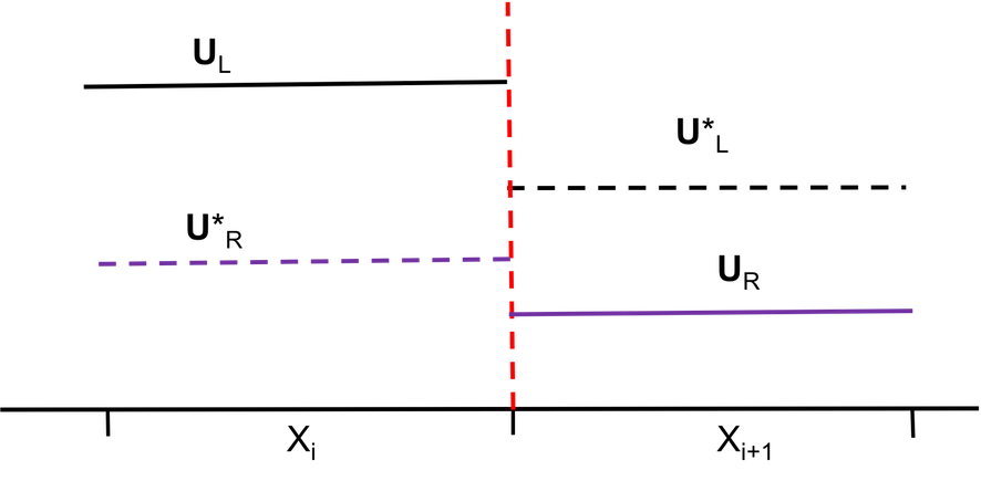
Sharp interface techniques is used in this study to resolve fine behaviours at the interface. Level set function is used to maintain the sharpness of the interface, and materials on either side of the interface are treated separately and therefore are evolved individually. To capture the correct interaction at the interface, I adopted the Riemann ghost fluid method, where a Riemann exact solver(iterative method) is used to solve for the intermediate state on either side of the interface. The intermediate states are the ghost fluid values for interfacial cells, which are then populated across the whole ghost fluid regions. A Riemann problem solution provides physically (thermodynamics) reasonable solutions for multi-materials at the interface as the contact discontinuity is the interface between the materials and this will be true for any systems of equations. As the graph shows, the Riemann problem based numerical methods use the solution at $ X_{1+\frac{1}{2}}$ to compute fluxes. For the left material and a Godunov update scheme, the correct $ U^ \ast _{L} $ state would be used to compute fluxes. To reproduce the left-moving wave structure along $ z _{i+\frac{1}{2}}$, we set the ghost fluid state at x to be \( U^ \ast _{R} \). This generates the right-moving wave and also has the correct speed of a generated contact.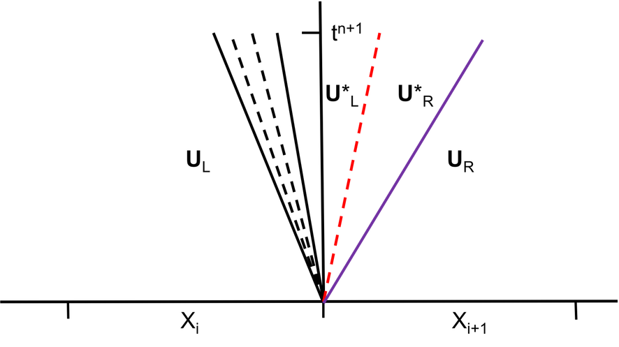
 In two dimensional test, in order to increase the accuracy of the ghost cell value, I adapted Sambasivan, 2000 approach that used a bilinear interpolation across the interface. This method uses four cells on either side of the interface to obtain the left and right state vectors. I implemented trans-missive boundary conditions to ensure the accuracy of the extrapolation at boundaries. Correct interpolation of left and right material becomes increasingly critical as the interface become less aligned with either axis. Dimensional splitting is used to update the state values with flux contribution from both x and y direction. The initial conditions is used for the first sweep in x direction for the time step $\Delta t $ , from which a update in x direction is obtained, which is then used for y sweep under the same time step $\Delta t $. The maximum time step that ensures the simulation stability is the minimum time step from both directions.
After obtaining ghost fluid values for interracial cells, I extrapolate these information into ghost fluid regions for all materials. The equation for constant extrapolation is:
\[\hat \cdot \nabla Q = 0\]
In two dimensional test, in order to increase the accuracy of the ghost cell value, I adapted Sambasivan, 2000 approach that used a bilinear interpolation across the interface. This method uses four cells on either side of the interface to obtain the left and right state vectors. I implemented trans-missive boundary conditions to ensure the accuracy of the extrapolation at boundaries. Correct interpolation of left and right material becomes increasingly critical as the interface become less aligned with either axis. Dimensional splitting is used to update the state values with flux contribution from both x and y direction. The initial conditions is used for the first sweep in x direction for the time step $\Delta t $ , from which a update in x direction is obtained, which is then used for y sweep under the same time step $\Delta t $. The maximum time step that ensures the simulation stability is the minimum time step from both directions.
After obtaining ghost fluid values for interracial cells, I extrapolate these information into ghost fluid regions for all materials. The equation for constant extrapolation is:
\[\hat \cdot \nabla Q = 0\]
which is very similar to the level set reinitialisation:
\[\hat \cdot \nabla \phi = 1\]In fact the techniques used for both are nearly identical. In this study, I used fast sweep approach to populate the ghost cell values. For ghost fluid boundary condition extrapolation, we use the level set function to determine the direction of the extrapolation, but compute gradients of the ghost fluid quantity instead.
\[P(Q_{i,j,k}) = ( \frac{ Q_{i,j,k} - Q_x}{\Delta x})^2 + ( \frac{ Q_{i,j,k} - Q_y}{\Delta y})^2 = 0\] The choice of \(Q_x\) and \(Q_y\) depends on the value of level set function (Sambasivan2009).Results and validation
| Test | \(\rho_L\) | \(u_L\) | \(p_L\) | \(\rho_R\) | \(u_R\) | \(p_R\) |
|---|---|---|---|---|---|---|
| 1 | 1.0 | 0.0 | 1.0 | 0.125 | 0.0 | 0.1 |
| 2 | 1.0 | -2.0 | 0.4 | 1.0 | 2.0 | 0.4 |
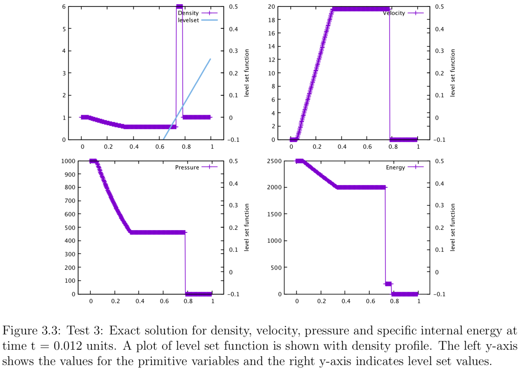
| 3 | 1.0 | 0.0 | 1000.0 | 1.0 | 0.0 | 0.01 |
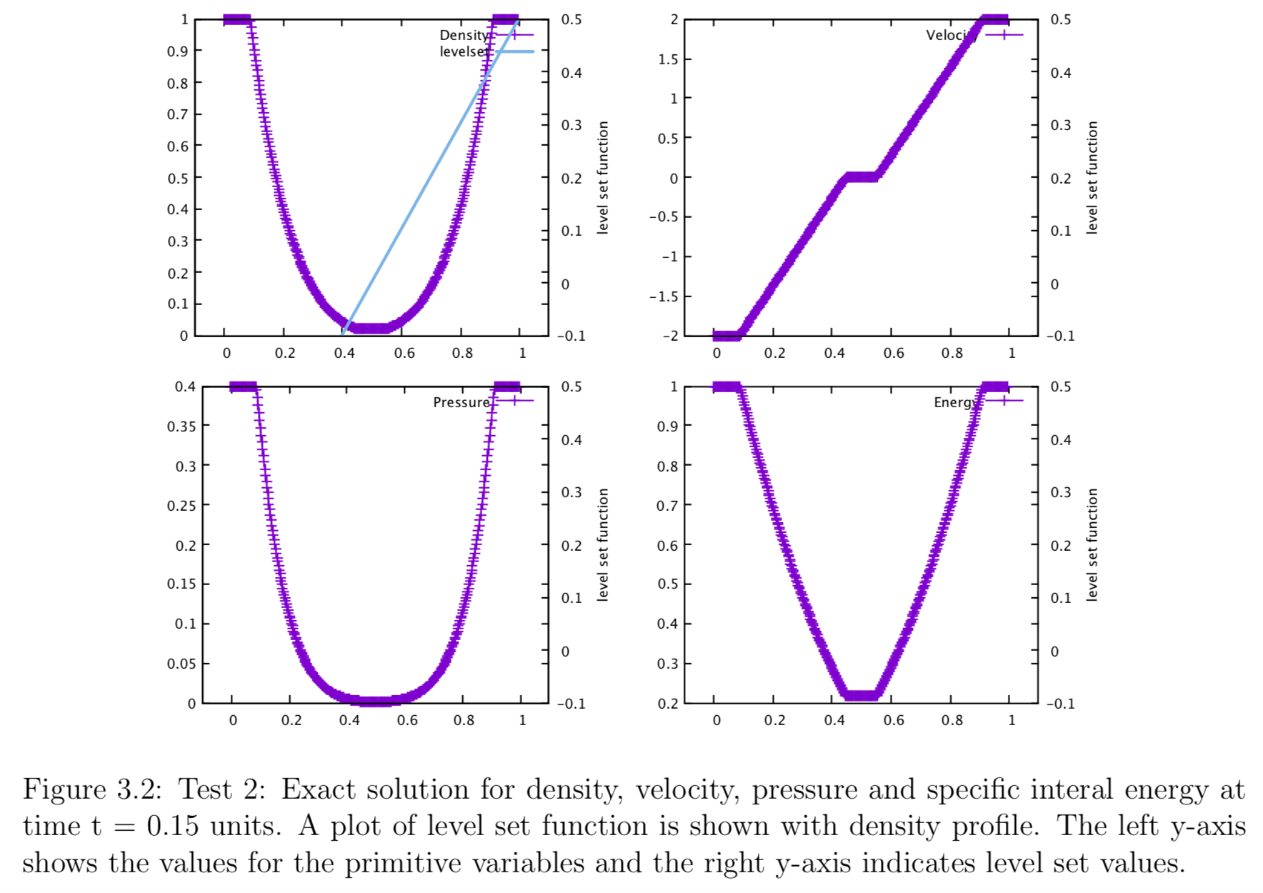
The Riemann-problem based ghost fluid method is first tested against three simulation with parameters shown in the table above. A level set function is used to mark the location of the contact discontinuity, where the state left and right have different values. Tests are taken from Toro2009. Test one is the famous Sod test problem. which has solutions consist of a left rarefraction, a contact and a right shock. Figures show the solution profiles for density, velocity, pressure and specific internal energy across the complete wave structure, at time t = 0.25 units. A plot of level set function is also shown along with the density profile. It has zero value at contact discontinuity, where is regarded as “multimaterial interface”. Due to the simplicity of the problem level set function takes the simplest form:
\[\phi = x - x_0\] where \( x_0\) is the location of the contact discontinuity \cite{Toro2009}. Test 2 is called the 123 problem, which has solutions consisting of two strong rare fractions and a stationary contact discontinuity. The test imposes difficulty on finding star state pressure ( i.e. \(p\ast\) ) as the pressure is very small (i.e. close to vacuum ), therefore testing the iterative method's stability. Test 2 is useful assessing the performance of numerical methods for low density flows. The level set function that is used track the shock location is plotted with density. The value is zero at the contact. Figure shows the density, velocity, pressure and internal energy profile at time = 0.15 units. Test 3 is a very severe test problem, the solution contains a left rarefraction, a contact and a right shock. It can be regarded as the propagation of a blast wave from right to left. The thrid figure shows the density, velocity, pressure and internal energy profile at time = 0.0012 units. The numerical simulation is conducted using Riemann problem-based ghost fluid method, with an exact solver (iterative scheme). level set function evolves with a simple advection equation (i.e. a form of Hamilton-Jacobi equation). The location of contact discontinuity can be interpolated from the function. It is where level set function equals zero (i.e. where the function crosses the x axis, \( \phi = 0.0 \)). Two states of material are treated separately (i.e. two separate simulation domains). At the contact, I implement Riemann problem based ghost fluid method where a Riemann problem will be solved to obtain the star states for the conservative variables either side of the contact discontinuity. These intermediate states are then populated into the ghost fluid regions of the two simulation domains. Then I applied Riemann exact solver to evaluate two simulation domain to obtain the profile at final time. The Level set function is then used to find the new location of the contact, which is used to combine the updated left and right states. This test is not a true multimaterial tests, nonetheless, by treating the contact discontinuity as a material interface, one can test if the ghost fluid method has been correctly implemented for the simplest scenario. Figures below show the solution profiles for density, pressure, velocity and specific internal energy for test 1, 2, 3 respectively. Location of the final contact discontinuity is interpolated from level set function as it takes a value of zero.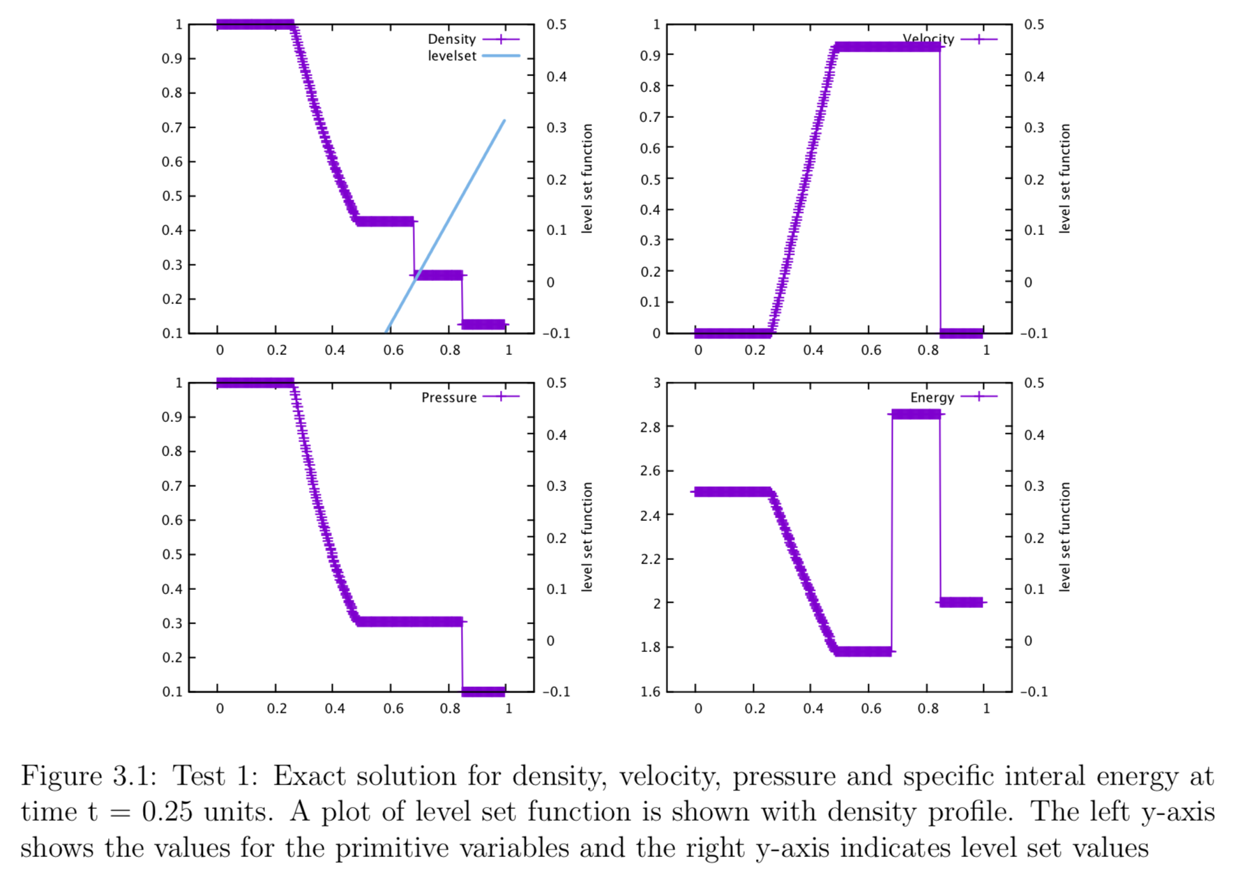
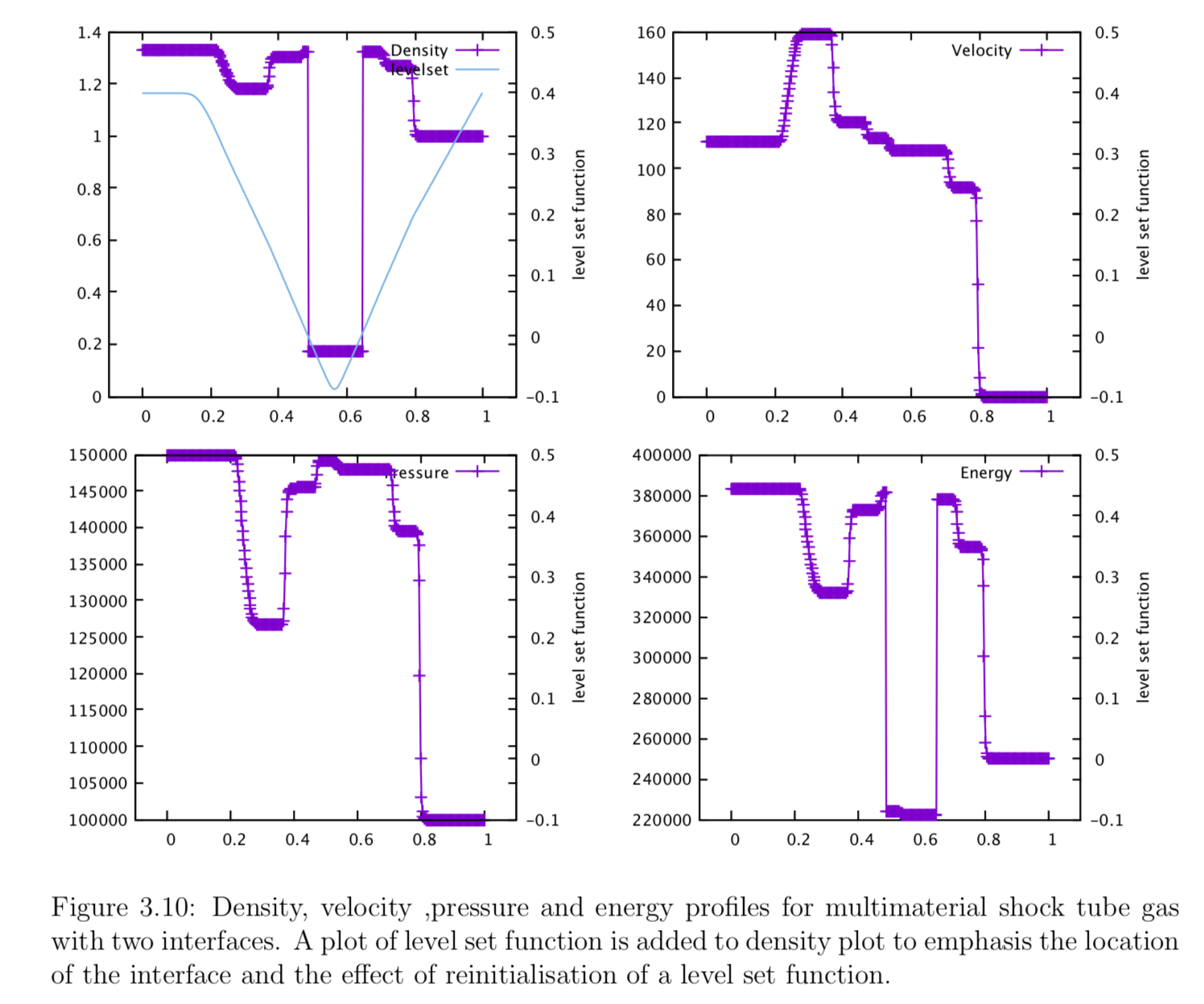
Multimaterial shock tube for gases with two interfaces
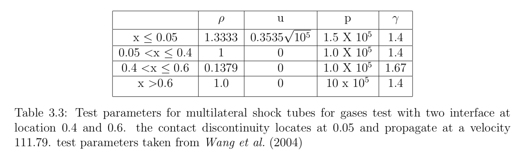
Table above shows the test parameters for the multimaterial shock tube for gases with two interfaces. This test consider a small region of helium with adiabatic exponent equal to 1.67. The results are obtained using the a second-order Godunov method, namely MUSCL-Hancock with HLLC solver and super-bee slope limiter. For a simulation domain with 400 cells, the first interface locates in between cell 160 and 161 while the second interface locates in between 240 and 241. The initial contact discontinuity propagates from cell 20 toward the two interfaces. The test is ran till 0.0014 such that all features are visible \cite{Wang2004}. The Riemann problem based ghost fluid methods preserved the sharp material interfaces and enabling accurate simulation near the interface. Since the presence of two material interfaces, the level set equation takes the form:
\[\phi = max( (x - x_1), (x_2 - x))\]where \(x_1\) and \(x_2\) are the interface locations.
Figure below shows the density, velocity, pressure and energy profiles across the domain. Level set function is plotted with the density profile. There is no spurious oscillations in all plots. Air’s density profile shows three distinctive features to the left of the interface: a rarefraction followed by a shock wave and a small rarefraction near the interface. In helium, all wave structure disappear from density profiles, however, a small rarefraction is seen from other profiles. To the right of the second interface, there is another rarefaction and shock wave seen in air.
The level set function is ploted with the density profile. Level set function has zero values at interface, Reinitialisation is applied to revert the general level set equation to a sign distance function, therefore reducing simulation error and steepening resembles a discontinuity.
References
- Toro, E. F. (2009), Riemann Solvers and Numerical Methods for Fluid Dynamics, thrid ed., Springer.
- Sambasivan, S. K., and H. S. UdayKumar (2009), Ghost fluid method for strong shock interac- tions part 1: Fluid-fluid interfaces, AIAA Journal, 47 (12), 2907–2922
- Wang, C. W., T. G. Liu, and B. C. Khoo (2006), A real ghost fluid method for the simulation of multimedium compressible flow, SIAM Journal on Scientific Computing, 28(1), 278–302