
HLLC Solver for Riemann problems for Fluid Dynamics -Ghost Fluid Method Serie 1
HLLC Solver uses Godunov flux to resolve shock wave emerged from hyperbolic PDEs. This finiste volume method ensure the conservative nature.
In this study, I investigated the techniques of Riemann ghost fluid method in solving the compressible multimaterial unsteady Euler equations. The study used MUSCL-Hancock with Super-bee slop limiter and HLLC as the approximate Riemann problem solver. Simulations are completed for single material shock tube test with a contact discontinuity, multimaterial shock tube test with a single and two interfaces. The later is also extended into two dimension with interface aligned with x and y axis, as well as having an angled with x axis. In addition, I have also investigated the effect of level set function reinitialisation using Mach 10 shock. The study confirmed the effectiveness of Riemann ghost fluid method in resolving the sharp interface and capturing the fine behaviour close to the interface. In addition, The use of second order numerical method that is also total variation diminishing ensuring high resolution and no presence of spurious oscillation. To be able to ensure an accurate representation of material interface, reinitialisation of the level set function is necessary. It also reduced dissipation cause by steepening, therefore reducing numerical error at the interface.
The Equations of Fluid Dynamics
Euler's Equations
In this study, I consider the time-dependent Euler Equations. These are systems of non-linear hyperbolic equations obeying conservation law, describing the dynamics of compressible material. In comparison with original Navies-Stoke equations, the effect of gravity, viscosity and body forces are neglected The five governing conservation laws are:
\[\rho_{t} + ( \rho u )_{x} + (\rho v)_{y} + (\rho w)_{z} = 0.\] \[(\rho u)_{t} + ( \rho u^2 + P )_{x} + (\rho u v)_{y} + (\rho u w)_{z} = 0.\] \[(\rho v)_{t} + ( \rho u v )_{x} + (\rho v^2 + p)_{y} + (\rho u w)_{z} = 0.\] \[(\rho w)_{t} + ( \rho u w )_{x} + (\rho v w)_{y} + (\rho w^2 + P)_{z} = 0.\] \[E_{t} + (u(E+p)_{x} + (v(E+p))_{y} + (w(E + p))_{z} = 0.\]I used primitive variables to describes the flow under consideration, namely, \( \rho(x, y, z,t) = \) density or mass density, \( p(x,y,z,t) = \) pressure, \( u(x,y,z,t) = \) x-component of velocity, \( v(x,y,z,t) = \) y-component of velocity, \( w(x,y,z,t) = \) z-component of velocity and E is the total energy per unit volume.
\[E = \rho (\frac{1}{2 \textbf(V)^2 + e})\]where \(\frac{1}{2}\textbf(V)^2 = \frac{1}{2}\textbf(V) \cdot \textbf(V) = \frac{1}{2}(u^2 + v^2 + w^2)\) is the specific kinetic energy and e is the specific internal energy.
Thermodynamic consideration and equation of states
The state governing equation (i.e. Euler’s equation) for the dynamics of a compressible material are insufficient to completely describe the physical processes involved. There are more unknowns than equations, therefore a closure condition is required. Such closing condition can be described by an equation of state. A system in thermodynamic equilibrium can be completely described by the basic thermodynamic variables pressure $p$ and specific volume v. As two materials involved in the simulation are thermally ideal gases therefore the relationship between thermodynamic variables p, v, T take the simple expression:
\[T = \frac{pv}{R}\]where (R) is a constant depending on the particular gas under consideration. The first law of thermodynamics states that for a non-adiabatic system the change in internal energy in a process will be given by
\(\Delta e = \Delta W + \Delta Q\)
The first law of thermodynamics can be written as :
\[dQ = de + pdv\]For a calorically ideal gas the internal energy $e$ can be related to p and v via a caloric equation of state which has the simple expression:
\[e = \frac{pv}{\gamma -1} = \frac{P}{\rho(\gamma -1)}\]The caloric equation state is sufficient to close the system for the Euler equations, unless temperature $T$ is needed, in which case a thermal EOS needs to be given explicitly .
Numerical Solutions for Hyperbolic Equations
Hyperbolic Partial Differential Equations (PDEs) are time-dependent problems without dissipation. For such problems, discontinuity may form from smooth initial conditions. Therefore we often need to obtain solutions from a Riemann problem. A Riemann problem is defined as a specific initial value problem composed of a conservation law together with piece wise constant initial data which has a single discontinuity. For the propose of solving compressible Euler equation, HLLC approximate Riemann Solvers was used.
The HLLC Riemann Solve
The approximate Riemann solver proposed by Harten Lax and Van leer (HLL) were later modified by Toro to form what is known as the HLLC (C stands for Contact) . HLLC adopts a three-waves model for the structure of the exact solution. Simulation resolution is improved via an incorporation of an intermediate wave. Figure below shows the three waves representation of a Riemann problem where four regions of solutions were separated by three waves with velocity \(S_{L}\), \(S_{*}\) and \(S_R\). They correspond to velocity for the left, intermediate and right wave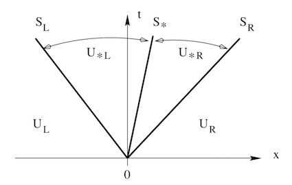
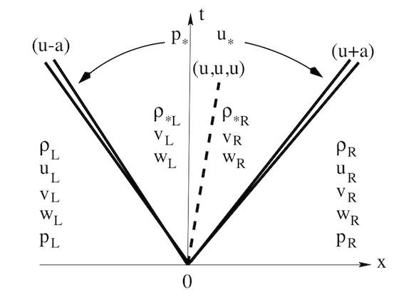
Through some algebraic manipulation, we found the intermediate the intermediate wave velocity as:
\[S_{*} = \frac{p_R - p_L +\rho_L u_L(S_L - u_L) - \rho_R u_R (S_R - u_R)}{\rho_L(S_L - u_L) - \rho_R(S_R - u_R)}\] fluxes \textbf{F}_{\ast L} and \textbf{F}_{\ast R} are related to fluxes on either side as : \[\textbf{F}_ {\ast K} = \textbf{F}_{K} + S_K(\textbf{U}_{\ast K} - \textbf{U}_K)\] for \(K = L\) or \( K = R\), with the intermediate states given as \[\textbf{U}_{\ast K}= \rho_K (\frac{S_K - u_K}{S_K - S_\ast}) \begin{bmatrix} 1\\ S_\ast \\ v_K\\ w_K\\ \frac{E_K}{\rho_K} + (S_\ast - u_K)[S_\ast + \frac{p_K}{\rho_K(S_K - u_K)}] \end{bmatrix} \label{intermediate state vector}\]where the left and right speed are obtained using pressure based wave-speed estimate .
References
- Harten, A., P. D. Lax, and B. van Leer (1983), On Upstream Differencing and Godunov- Type Schemes for Hyperbolic Conservation Laws, SIAM Review, 25(1), 35–61
- Toro, E. F. (2009), Riemann Solvers and Numerical Methods for Fluid Dynamics, thrid ed., Springer.
- Toro, E. F., M. Spruce, and W. Speares (1994), Restoration of the contact surface in the HLL-Riemann solver, Shock Waves, 4 (1), 25–34,